First of all, I can recommend everyone writting a blog, because its a greate way of self relfection of the learned stuff.
What is a Spikin Neural Network?
Spiking Neural Networks (SNN) are the 3rd generation of neural networks.
What are first generation NNs?
1st gen. NNs are based on McCulloch-Pitts threshold neurons and are a very simple model from the year 1943. A neuron sends a binary „on“ signal if the weighted sum of all incoming signals is above a specific \(\theta\). Be aware, the output of this neuron is NOT linear!
What are second generation NNs?
2nd gen. NNs are NOT based on the non-linear threshold function described above but use a linear continuous activation function. Many of them are still discussed by various papers and blogs: sigmoid, tanh are the famous one! Be aware: in some cases the activation function is still non-linear, just think about ReLU (\(f(x) = max(0, x)\) where a better function would be the softplus: \(f(x) = ln(1 + e^x)\))
3rd generation NNs
Now we face 3rd generation NNs. The neurons in these networks are using again the binary outputs from the 1st gen nets. But the big difference is that one neuron does not send out only one such a „signal“, it sends out many of them. They are so called „spike trains“. This model is somehow similar to the functionality of our brain’s neurons. Our human neurons continuously send out „spikes“. One side node here: one human neuron receives spikes from up to 10.000 neurons and sends spikes to another 10.000 neurons via so called dendrites – the connection between two neurons (simplified). Those dendrites for sure have a length and in our brain we have up to 4 kilometres of them in EVERY cubic millimetre. Whether they are very small but they are one of the most complex parts of our body. Beside that back to a spike train. So we have a neuron \(i\) which sends such a train. One spike at a specific timestep \(t^i\) in a train is a „1“ signal. Now we can encode this into a set \(F_i\) which is the spike train for neuron \(i\) with \(F_i = \{t^1, …, t^n\}\). Further: a spike is sent if the neuron \(i\)’s potential is reaching a certain threshold \(\vartheta\). So a timestamp \(t_j \in F_i \Leftrightarrow u_i(t_j) \geq \vartheta\). Moreover we have to ensure that the neurons potential is further increasing. To define this we add \(u_i'(t_j) > 0\) as condition since \(u(t)\) will increase if the first derivative \(u'(t) > 0\). So we can define now \(F_i = \{ t | u_i(t) \geq \vartheta \land u_i'(t) > 0 \}\). (Note: This is now simple: if \(t \in F_i\) then neuron \(i\) fires at \(t\)).
How does such a spike train look like in reality? Here you have a measurement recording from such an investigation:
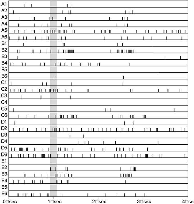
Here you see some neurons on the left side, sending out spikes. The interesting thing here is that the x-axis defines the time and we can see how the neurons behave during the time.
So we have to distinguish between two values: the internal state or the membran potential AND the action potential. When the internal state reaches the threshold it comes in the phase of „absolute refractoriness“. In this phase the internal state reaches a high level of energy and after words it comes to a „reload“ phase. This phase is the relative refractoriness. So if the internal state rises above the previously described threshold, the action potential is 1 otherwise 0. The following diagram shows the internal state of a neuron when it reaches the threshold (0):

In this diagram it can be seen that the internal state reaches a high level (absolute refractoriness) and decrases to reload (relative refractoriness). The formula is: \(\eta(s) = -n_0 * e^{-\frac{s-\delta^{abs}}{t}}*H(s – \delta^{abs})-K*H(s)*H(\delta^{abs}-s)\) and \(H(x)\) returns 1 if \(x > 0\) otherwise 0.
Done in Octave with:
f = figure();
function y = H(x)
  y = double(x > 0)
endfunction
function y = eta(s)
  t = 0.1
  deltaabs = 0.02
  K = -0.2
  n0 = 0.1
  y = -n0 .* exp(-(s - deltaabs) ./ t) .* H(s - deltaabs) - K .* H(s) .* H(deltaabs - s)
endfunction
hold on;
clf
s = 0:0.005:0.5;
plot(s, eta(s), "linewidth", 2);