In medias res: We skip the whole intro about „how great music is and that it touches everyone“ and so on and write about the topic. We coded a first draft of a music note detector in python. We defined two requirements:
- We have the list of frequencies for the notes available
- We use an existing implementation of FFT (scipy.fft.fft)
We want to clarify that this is a first draft and there is a big optimization potential. But we wanted to know how fast we could implement such a detector.
Further we expect the basic knowledge from FFT and (not required but recommended) equally tempered tunic system.
Coming to the first point from above – the list of frequencies with their corresponding music notes label is derived from the „equally tempered“ twelve tone tuning system:
notes = [
    ['C0', 16.35, []],
    ['C#0/Db0', 17.32, []],
    ['D0', 18.35, []],
    ['D#0/Eb0', 19.45, []],
    ['E0', 20.60, []],
    ['F0', 21.83, []],
    ['F#0/Gb0', 23.12, []],
    ['G0', 24.50, []],
    ['G#0/Ab0', 25.96, []],
    ['A0', 27.50, []],
    ['A#0/Bb0', 29.14, []],
    ['B0', 30.87, []],
    ['C1', 32.70, []],
    ['C#1/Db1', 34.65, []],
    ['D1', 36.71, []],
    ['D#1/Eb1', 38.89, []],
    ['E1', 41.20, []],
    ['F1', 43.65, []],
    ['F#1/Gb1', 46.25, []],
    ['G1', 49.00, []],
    ['G#1/Ab1', 51.91, []],
    ['A1', 55.00, []],
    ['A#1/Bb1', 58.27, []],
    ['B1', 61.74, []],
    ['C2', 65.41, []],
    ['C#2/Db2', 69.30, []],
    ['D2', 73.42, []],
    ['D#2/Eb2', 77.78, []],
    ['E2', 82.41, []],
    ['F2', 87.31, []],
    ['F#2/Gb2', 92.50, []],
    ['G2', 98.00, []],
    ['G#2/Ab2', 103.83, []],
    ['A2', 110.00, []],
    ['A#2/Bb2', 116.54, []],
    ['B2', 123.47, []],
    ['C3', 130.81, []],
    ['C#3/Db3', 138.59, []],
    ['D3', 146.83, []],
    ['D#3/Eb3', 155.56, []],
    ['E3', 164.81, []],
    ['F3', 174.61, []],
    ['F#3/Gb3', 185.00, []],
    ['G3', 196.00, []],
    ['G#3/Ab3', 207.65, []],
    ['A3', 220.00, []],
    ['A#3/Bb3', 233.08, []],
    ['B3', 246.94, []],
    ['C4', 261.63, []],
    ['C#4/Db4', 277.18, []],
    ['D4', 293.66, []],
    ['D#4/Eb4', 311.13, []],
    ['E4', 329.63, []],
    ['F4', 349.23, []],
    ['F#4/Gb4', 369.99, []],
    ['G4', 392.00, []],
    ['G#4/Ab4', 415.30, []],
    ['A4', 440.00, []],
    ['A#4/Bb4', 466.16, []],
    ['B4', 493.88, []],
    ['C5', 523.25, []],
    ['C#5/Db5', 554.37, []],
    ['D5', 587.33, []],
    ['D#5/Eb5', 622.25, []],
    ['E5', 659.25, []],
    ['F5', 698.46, []],
    ['F#5/Gb5', 739.99, []],
    ['G5', 783.99, []],
    ['G#5/Ab5', 830.61, []],
    ['A5', 880.00, []],
    ['A#5/Bb5', 932.33, []],
    ['B5', 987.77, []],
    ['C6', 1046.50, []],
    ['C#6/Db6', 1108.73, []],
    ['D6', 1174.66, []],
    ['D#6/Eb6', 1244.51	, []],
    ['E6', 1318.51, []],
    ['F6', 1396.91, []],
    ['F#6/Gb6', 1479.98, []],
    ['G6', 1567.98, []],
    ['G#6/Ab6', 1661.22, []],
    ['A6', 1760.00	, []],
    ['A#6/Bb6', 1864.66, []],
    ['B6', 1975.53	, []],
    ['C7', 2093.00, []],
    ['C#7/Db7', 2217.46, []],
    ['D7', 2349.32, []],
    ['D#7/Eb7', 2489.02, []],
    ['E7', 2637.02, []],
    ['F7', 2793.83, []],
    ['F#7/Gb7 ', 2959.96, []],
    ['G7', 3135.96, []],
    ['G#7/Ab7', 3322.44, []],
    ['A7', 3520.00, []],
    ['A#7/Bb7', 3729.31, []],
    ['B7', 3951.07, []],
    ['C8', 4186.01, []],
    ['C#8/Db8', 4434.92, []],
    ['D8', 4698.63, []],
    ['D#8/Eb8', 4978.03, []],
    ['E8', 5274.04, []],
    ['F8', 5587.65, []],
    ['F#8/Gb8', 5919.91, []],
    ['G8', 6271.93, []],
    ['G#8/Ab8', 6644.88	, []],
    ['A8', 7040.00, []],
    ['A#8/Bb8', 7458.62, []],
    ['B8', 7902.13, []],
]
The list is pretty clear: The first index of each row defines the label of the note, the second one defines the frequency and the third one is a prepared array for meta data which we won’t need here in this demo.
We record 100ms into a WAV file via pyaudio and then pass this file to the FFT to grab the frequencies spectrum. We read the WAV file with: scipy.io.wavfile
    audio = pyaudio.PyAudio()
    stream = audio.open(format=FORMAT, channels=CHANNELS,
                    rate=RATE, input=True,
                    frames_per_buffer=CHUNK)
    frames = []
    for frameIndex in range(0, int(RATE / CHUNK * RECORD_SECONDS)):
        data = stream.read(CHUNK)
        frames.append(data)

    stream.stop_stream()
    stream.close()
    audio.terminate()

    waveFile = wave.open(WAVE_OUTPUT_FILENAME, 'wb')
    waveFile.setnchannels(CHANNELS)
    waveFile.setsampwidth(audio.get_sample_size(FORMAT))
    waveFile.setframerate(RATE)
    waveFile.writeframes(b''.join(frames))
    waveFile.close()
Our configuration for the parameters:
FORMAT = pyaudio.paInt16
CHANNELS = 2
RATE = 88200
CHUNK = 5012
RECORD_SECONDS = 0.1
WAVE_OUTPUT_FILENAME = "file.wav"
We use the FFT implementation scipy.fft.fft for our use case. And the magic happens here:
    fileSampleRate, signal = wavfile.read("file.wav")
    if len(signal.shape) == 2:
        signal = signal.sum(axis=1) / 2
    N = signal.shape[0]
    seconds = N / float(fileSampleRate)
    timeSamplesPerSecond = 1.0 / fileSampleRate
    timeVector = scipy.arange(0, seconds, timeSamplesPerSecond)
    fft = abs(scipy.fft.fft(signal))
    fftOneSide = fft[range(N // 2)]
    fftFrequencies = scipy.fftpack.fftfreq(signal.size, timeVector[1] - timeVector[0])
    fftFrequenciesOneSide = fftFrequencies[range(N // 2)]
We simply call the FFT function and grab out the frequencies. Since we get a symmetric spectrum (left channel and right channel) we remove one side.
Further we simply calculated the x and y values for the diagrams here:
realAbsoluteValues = abs(fftOneSide)
normalizedAbsoluteValues = abs(fftOneSide) / np.linalg.norm(abs(fftOneSide))
x = []
y = []
yRealValues = []
recordedNotes = []
for frequencyIndex in range(0, len(fftFrequenciesOneSide)):
    if fftFrequenciesOneSide[frequencyIndex] >= 110 and fftFrequenciesOneSide[frequencyIndex] <= 8200:
        x.append(fftFrequenciesOneSide[frequencyIndex])
        y.append(normalizedAbsoluteValues[frequencyIndex])
        yRealValues.append(realAbsoluteValues[frequencyIndex])
        if normalizedAbsoluteValues[frequencyIndex] > 0.25:
            note = getNote(fftFrequenciesOneSide[frequencyIndex])
            if note != '':
                generalizedNote = normalizeNote(note)
                if generalizedNote not in recordedNotes:
                    recordedNotes.append(generalizedNote)
print(recordedNotes)
The rest is simple data displaying now:
    plt.subplot(411)
    plt.plot(timeVector, signal, "g")
    plt.xlabel('Time')
    plt.ylabel('Amplitude')
    plt.subplot(412)
    plt.plot(fftFrequencies, fft, "r")
    plt.xlabel('Frequency (Hz)')
    plt.ylabel('Count dbl-sided')
    plt.subplot(413)

    plt.plot(x, y, "b")
    plt.xlabel('Frequency (Hz)')
    plt.ylabel('Count single-sided')
    plt.subplot(414)
    plt.plot(x, yRealValues, "b")
    plt.xlabel('Frequency (Hz)')
    plt.ylabel('Count single-sided')
    plt.show()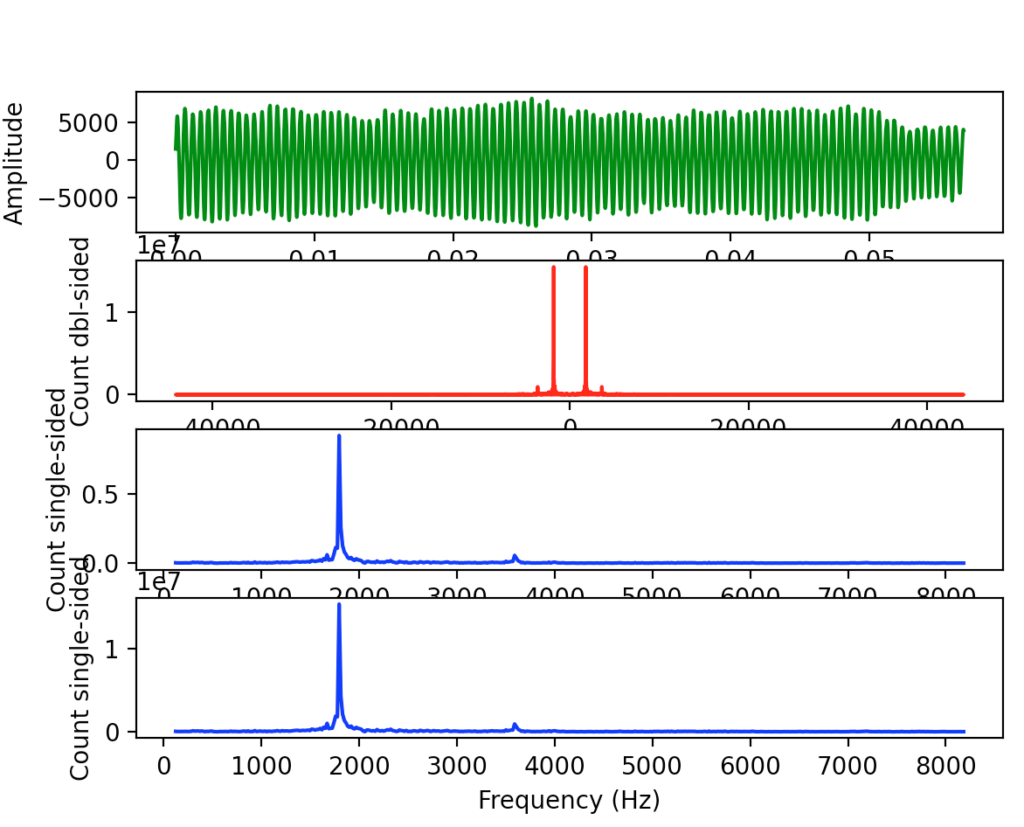
As you can see the first is the amplitude which is great a „good“ one because it seems to be clear.
In the 2nd diagram you can see that we can a 2 sided spectrum so we can remove one side.
We defined two functions:
def normalizeNote(note):
    if len(note) == 2:
        return note[0]
    else:
        return note[0] + note[1]
The previous one is only removing some „#“ suffixes from a note. E.g. you pass „B3“ and it will return „B“ or you pass „B#3“ and it will return „B#“. (Really primitive).
The second function is:
def getNote(frequency):
    global notes
    for noteIndex in range(0, len(notes)):
        noteData = notes[noteIndex]
        uppperBoundFrequency = noteData[1] * 1.015
        lowerBoundFrequency = e[1] * 0.986
        if frequency >= lowerBoundFrequency and frequency <= uppperBoundFrequency:
            return noteData[0]
    return ''
This one is also not sophisticated but a little bit of music knowledge is helpful here. Since not every note is perfectly pitched at the frequency where it should be and also some phrasings would skew the frequency of a note, an „epsilon“ area around a note is helpful to detect it. So basically the passed frequency is compared to a range where a specific note could be.
See the full source of the python3 source code here: https://github.com/mrqc/primitive-music-notes-detector/blob/main/pitch-det.py